A solar power tower plant uses flat, rotating mirrors called heliostats to reflect and concentrate solar radiation onto a tower-mounted receiver. Figure 1 shows heliostats reflecting sunlight during solar noon, when the sun is at its zenith in the sky.

Throughout the day, each heliostat rotates to ensure that the sunlight remains focused on the receiver by using a tracking system as shown in Figure 2.

Note that the position of the sun varies, and individual heliostats can be blocked or shaded by neighboring heliostats, which affects the efficiency of the power plant. In addition, there are other factors that affect the power plant’s efficiency as described in Table 1.
| Name | Description |
|---|---|
| Cosine effect | Loss due to the sun's rays not being perpendicular to the heliostat. |
| Spillage effect | Loss due to reflected rays missing the receiver. |
| Atmospheric attenuation | Loss due to atmospheric absorption. |
| Shading effect | Sun rays being blocked by neighboring heliostats heliostats. |
| Blocking effect | Reflected rays being blocked by neighboring heliostats. |
Given the specifications of the power plant, including the tower height and receiver dimensions, the task is to determine the optimal locations of heliostats that maximize the plant’s efficiency. This optimal arrangement of heliostats is referred to as optimal layout.
Following a brief introduction, a simplified model is presented for determining the optimal layout. The task of finding an optimal layout for a single heliostat is solved using only geometry. In the case of multiple heliostats, discretization and ray tracing are used to estimate the efficiency of a solar power plant taking into account shading and blocking effects. Then, the layout is optimized using Sequential Quadratic Programming (SQP).
Table of contents
- Introduction
- Optical model for a solar tower power plant
- Cosine effect
- Spillage effect
- Atmospheric attenuation
- Optimal position for a single heliostat
- Multiple heliostats
- Source code
- References
Introduction
Concentrating solar power systems such as solar tower power plants concentrate sunlight to produce electricity, offering a renewable energy production. However, the cost of electricity from these systems remain high compared to other renewable sources, as indicated in Figure 3.

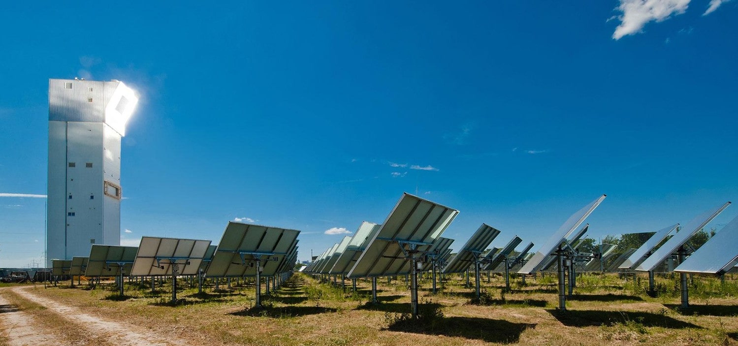
Efforts in research and development are focused on improving efficiency, cutting construction and operation expenses, and ultimately reducing electricity production costs. Figure 4 shows an experimental solar power tower plant at the German Aerospace Center.
Optical model for a solar tower power plant
We begin by examining a solar power tower plant employing a single heliostat and determining its optimal position. Although actual plants employ thousands of heliostats, focusing on a single one makes it easier to explain the model. Furthermore, the derived solution for a single heliostat allows us to verify the accuracy of the optimization methods to find the optimal layout for multiple heliostats. The model introduced here operates in two dimensions to simplify complexity, but a more realistic approach would involve replacing all definitions with their three-dimensional counterparts.
The normal $n(t)$ of heliostat at time $t$ is given by
\[\newcommand{\norm}[1]{\left\lVert#1\right\rVert} n(t) = \frac{r + s(t)}{\norm{r + s(t)}}.\]Here, $r$ denotes the direction from the center $H$ of the heliostat to the center of the receiver $R$, while $s(t)$ is the normalized solar vector at time $t$, as illustrated in Figure 5.

Cosine effect
The primary energy loss in a solar power plant occurs when sunlight does not strike the heliostat perpendicularly. The effective reflection area of the heliostat is reduced by the cosine of one-half of the angle between vectors $r$ and $s$. This phenomenon is known as the cosine effect:
\[\eta_{cos} = \cos{\left( \frac{\gamma}{2} \right)}\]where
\[\gamma = \angle (r, s).\]As depicted in Figure 6A, an $\eta_{cos}$ value approximately 0 indicates minimal power output, while an $\eta_{cos}$ value close to 1 signifies maximum power output (Figure 6B).

In order to determine the optimal position of the heliostat to maximize the power output, we will express the cosine effect $\eta_{cos}$ in terms of the heliostat’s center $H$. Let $\rho$ denote the angle between a line passing through the receiver’s center $R$ and the heliostat’s center $H$, and the horizontal line passing through $R$. Additionally, let $\phi$ denote the angle between the direction of sunlight and the ground’s horizontal plane, as shown in Figure 7.

In this simplified model, as the sun’s position changes throughout the day, the solar angle $\phi$ ranges from 0 to $\pi$. The angle $\gamma = \angle (r, s)$ can be expressed in terms of $\phi$ and $\rho$ as:
\[\phi = |\pi - \phi - \rho|\]and cumulative daily cosine effect can be expressed in terms of $\rho$ as:
\[\begin{equation} \eta_{cos}(\rho) = \int_{0}^{\pi} \cos \left( \frac{|\pi - \phi - \rho |}{2} \right) d\phi = 2 \left( \sin \left( \frac{\rho}{2} \right) + \cos \left(\frac{\rho}{2}\right) \right). \label{eq: cosine-effect} \end{equation}\]Spillage effect
Solely focusing on the cumulative daily cosine effect, the optimal position of the heliostat to maximize power output is directly underneath the receiver. This corresponds to $\rho = \pi/2$, as indicated by equation \ref{eq: cosine-effect}.
However, in this position, many reflected rays from the heliostat fail to reach the receiver at various times throughout the day as illustrated in Figure 8A.

This effect on the energy loss is known as spillage effect and can be defined as follows:
\[\eta_{spill} = \text{the proportion of rays that reach the receiver.}\]To derive the spillage effect $\eta_{spill}$, let $\tau$ be the angle between the line passing through the receiver’s surface and the ground’s horizontal plane, as shown in Figure 9.

Note that,
\[\begin{align*} \alpha &= \pi - \tau - \rho \\[.5em] \beta &= (\phi + \rho) / 2. \end{align*}\]By similarity and sine rule,
\[\begin{align*} \frac{|AQ|}{|AR|} &= \frac{|AP|}{|AH|} \\[.5em] \frac{|AR|}{\sin{\alpha}} &= \frac{|AH|}{\sin{\beta}} \end{align*}\]we can derive the spillage effect in terms of angles $\rho, \tau$ and $\phi$ as
\[\begin{equation} \eta_{spill} = \min \left( 1, \frac{|HP|}{|RQ|} \right) = \min \left( 1, \frac{\sin{(\pi - \tau - \rho)} }{ \sin{\left((\phi + \rho)/2\right)} } \right). \label{eq: spillage-effect} \end{equation}\]Note that, in our model, the angle $\tau \approx 80^{\circ}$ and it is a fixed constant because it is part of plant’s specification. Therefore $\eta_{spill}$ only varies with respect to $\phi$ and $\rho$.
Atmospheric attenuation
Another loss of energy is due to atmospheric attenuation. This loss depends on the distance $d$ between a heliostat and the receiver and assumes a visibility of 40 km. See (Richter, 2017) for more details.
Denote by $d$ the distance in meters from the center $H$ of the heliostat to the center of the receiver $R$:
\[\newcommand{\norm}[1]{\left\lVert#1\right\rVert} d = \norm{H - R}\]The atmospheric attenuation effect, shown in Figure 10, is given by the formula:
\[\eta_{aa}(d) = \begin{cases} 0.99321 - 1.176 \cdot 10^{-4} d + 1.97 \cdot 10^{-8} d^{2}, \quad d \leq 1000 \, m\\ \exp(-1.106 \cdot 10^{-4} d), \quad d > 1000 \, m \end{cases}\]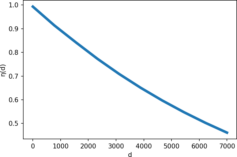
Optimal position for a single heliostat
To determine the optimal position for the center $H(\rho, d)$ of a single heliostat we define the following objective function called daily energy production of a power plant:
Daily Energy Production (DEP)
\[\text{DEP}(\rho, d) = \frac{1}{\pi} \, \eta_{aa}(d) \, \int_{0}^{\pi} \eta_{cos}(\rho, \phi) \, \eta_{spill}(\rho, \phi) \, d\phi\]
Note:
-
The normalizing constant is $1/\pi$ because when there are no losses, all effects are 1 and $\int_{0}^{\pi} d\phi = \pi$.
-
In this simplified model, as the sun’s position changes throughout the day, the solar angle $\phi$ ranges from 0 to $\pi$. This is why we integrate over $\phi$ from 0 to $\pi$.
To determine the optimal position for $H(\rho, d)$ that maximizes DEP, we need to find the optimal distance $d^{*}$ and optimal angle $\rho^{*}$.
Since $\eta_{aa}(d)$ is a monotonically decreasing function,
\[\DeclareMathOperator*{\argmin}{arg\,min} d^{*} = \argmin_{d} \norm{ H - R } \quad \text{ subject to: } \norm{ H - R } > 4 \, m.\]In our model, the heliostat and receiver are both 4 meters in size and the rotation of heliostats adds a constraint $\norm{ H - R } > 4 \, m.$ (See Figure 11B.) Therefore, the optimal distance is $d^{*} = 4 \, m$.
Plugging into DEP the derived equations \ref{eq: cosine-effect} and \ref{eq: spillage-effect} for $\eta_{cos}$ and $\eta_{spill}$ and integrating, we get DEP with respect to $\rho$ shown in Figure 11A. The optimal angle $\rho$ is approximately $30^{\circ}$.
The optimal position for a single heliostat is shown in Figure 11B.

Multiple heliostats
Shading and blocking effects
In case of multiple heliostats, individual heliostats can be blocked or shaded by neighboring heliostats, which affects the efficiency of the power plant (Figure 12). The effects of shading and blocking are defined as
\[\begin{align*} \eta_{shade} &= \text{ proportion of incoming rays not shaded by neighboring heliostats} \\[.5em] \eta_{block} &= \text{ proportion of reflected rays not blocked by neighboring heliostats}. \end{align*}\]
Discretization and ray tracing
Finding the optimal layout using only geometry is challenging when there are multiple heliostats.Therefore, discretization and ray tracing are used to estimate the reflected power of each heliostat that is hitting the receiver.
For each heliostat, we divide the surface of the heliostat into equal-area regions. We then trace a ray from each region in the direction of the sun and in the direction of the receiver. Figure 13 shows ray tracing for $m = 5$ rays.

Denote by $m$ the number of rays per heliostat and by $\eta_{ray, i}$ the proportion of rays that are received at the surface of heliostat $i$ and hit the surface of the receiver.
The layout optimization problem
For a given plant with $n$ heliostats with centers:
\[H_{1}, H_{2}, \dots, H_{n}\]we approximate the daily energy production by
\[\widehat{\text{DEP}}(H_{1}, H_{2}, \dots, H_{n}) = \frac{1}{n \, m} \sum_{i = 1}^{n} \eta_{aa, i} \, \sum_{k = 1}^{m} \eta_{cos, i}(\phi_{k}) \, \eta_{ray, i}.\]We can now define the layout optimization problem in a more formal manner.
Layout optimization problem
Determine the locations $H_{i}$ of heliostats $i = 1, 2, \dots, n$, that maximize the $\widehat{\text{DEP}}$ subject to:
- all $H_{i}$ are in the specified field area,
- all $H_{i}, H_{j}$ where $i \neq j$ are at least $4$ meters appart,
- $H_{i}, R$ are at least $4$ meters appart.
An example of a valid layout for $n = 5$ heliostats is in Figure 14. Here the field area is specified as follows. Maximum distance from receiver’s center to a heliostat’s center is 35 meters and maximum height of heliostat’s center is 10 meters.

Solving the layout optimization problem
Note that the objective function $\widehat{\text{DEP}}$ is not convex as indicated by Figure 15. It shows the plot of $\widehat{\text{DEP}}$ as we vary the location of $H_{3}$ in the layout shown in Figure 14.
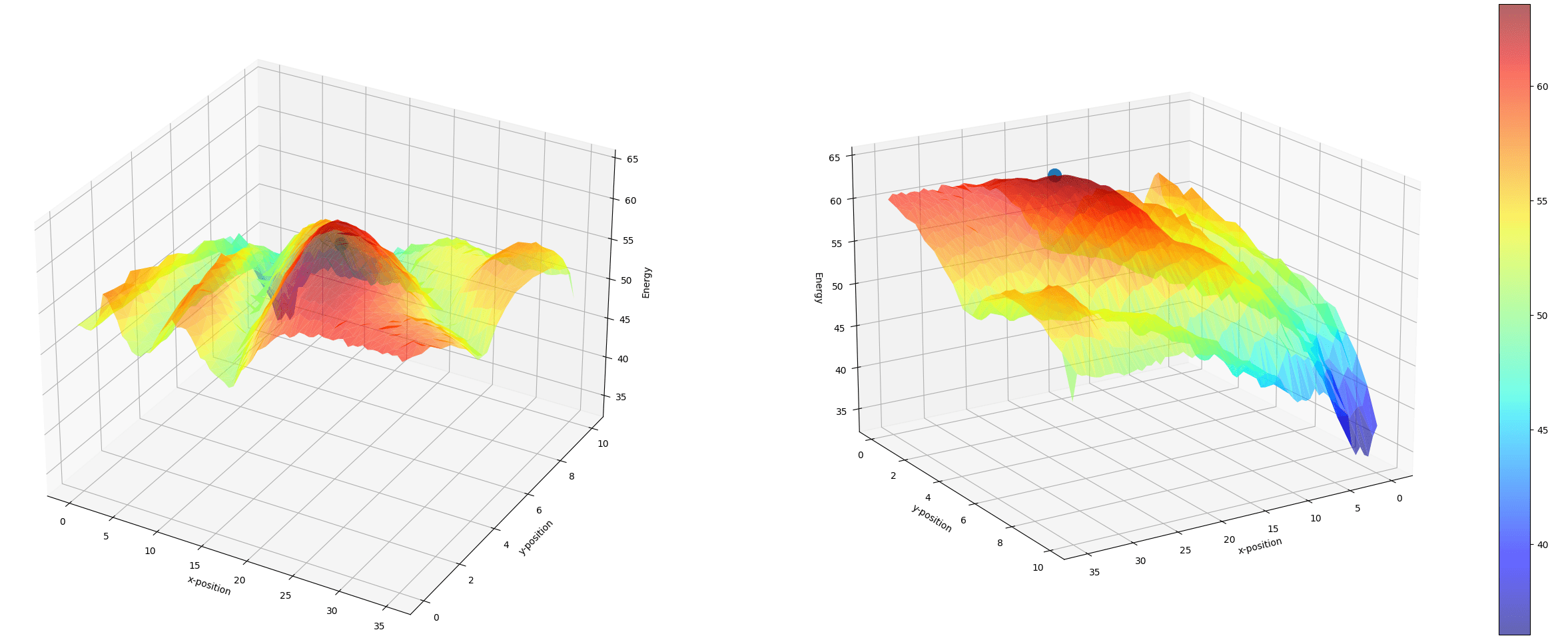
Starting far from the global optimum and running a gradient ascent can lead us to a sub-optimal solution. Similarly with higher order methods. Despite this, we can still observe some interesting results.
Example
Running Sequential Quadratic Programming (SQP) method from a class of Lagrange-Newton methods starting from some initial layout with 3 heliostats, the method converges to the layout show in Figure 16. See the Source code for more details.

It places the heliostats some distance appart on the parabola with focal point $R$:
\[y = \frac{1}{48} x^{2}.\]The layout we get for $n=5$ heliostats is shown in Figure 1. Intuitively this seems to be the best option. Generally speaking, the heliostats do not need to rotate so much to reflect the rays towards the receiver. Furthermore, the heliostats should be far apart in order to minimize the effects of shading and blocking. In particular, the effects of shading and blocking are most noticable when the cosine effect is minimized, that is when $\phi$ is roughly 90 degrees. In Figure 17 is sketch of the shadow from heliostat $H_{j}$ considering the values of $\phi$ close to 90 degrees.

Source code
The repository containing all Python scripts is available here:
The code for Example above:
import sys
import numpy as np
from scipy import optimize

# load the specifications of the plant
hypo_plant = utils.load("./data/plants/tiny-plant.json")

# set the initial layout
basic_layout = np.array([[10, 10], [20, 5], [30, 10]])
x0 = basic_layout.flatten()

# objective function
def f(x):
    plant.layout = x.reshape((3, 2))
    plant.set_layout()
    return -utils.get_energy(plant)

# set the bounds and constraints
bounds = []
for i in range(3):
    bounds.append((0, 35))
    bounds.append((0, 10))

def g01(x):
    i, j = 0, 1
    layout = x.reshape(3, 2)
    distance = np.linalg.norm(layout[i] - layout[j])
    return distance - 4

def g02(x):
    i, j = 0, 2
    layout = x.reshape(3, 2)
    distance = np.linalg.norm(layout[i] - layout[j])
    return distance - 4

def g12(x):
    i, j = 1, 2
    layout = x.reshape(3, 2)
    distance = np.linalg.norm(layout[i] - layout[j])
    return distance - 4

constraints = [{"type": "ineq", "fun": g01},
               {"type": "ineq", "fun": g02},
               {"type": "ineq", "fun": g12}]

result = optimize.minimize(f, x0,
                           method="SLSQP",
                           bounds=bounds,
                           constraints=constraints,
                           options={'disp': True, 'maxiter': 100})
# Optimization terminated successfully    (Exit mode 0)
#             Current function value: -41.033956692960274
#             Iterations: 28
#             Function evaluations: 317
#             Gradient evaluations: 28
References
- Richter, P. (2017). Simulation and optimization of solar thermal power plants [PhD thesis, RWTH Aachen University]. https://doi.org/10.18154/RWTH-2017-05351